AI and fluid dynamics

During my bachelor I was learning about computational fluid dynamics and programming in my Heat Transfer classes. After exploring popular methods such as the finite element method and finite volume method, I studied and programmed a simulator for the lattice Boltzmann method in Python.

Challenged by the high amount of time required to compute large simulations, despite an optimized setup, I decided to experiment with another topic of my interest: deep learning. For my thesis I proposed and elaborated a deep learning model using the simulator data which ran faster with accurate physical results.

Github project

lattice boltzmann method

The Lattice Boltzmann Method (LBM) is a computational fluid dynamics method for fluid simulation. Much like Conway's Game of Life , it is based on the concept of cellular automata.

The fluid is represented by a grid of cells, where each cell contains information about the fluid velocity distribution. The simulation is then computed by updating the cells according to the rules of the LBM.

a fluid simulation showing the coalescence of water drops — Example of LBM simulation with multiple phases.

Like Game of Life, it has rules that are applied after each frame, in particular, these are the equations that represent them Collision equation:

the lattice boltzmann collision equation

Streaming equation:

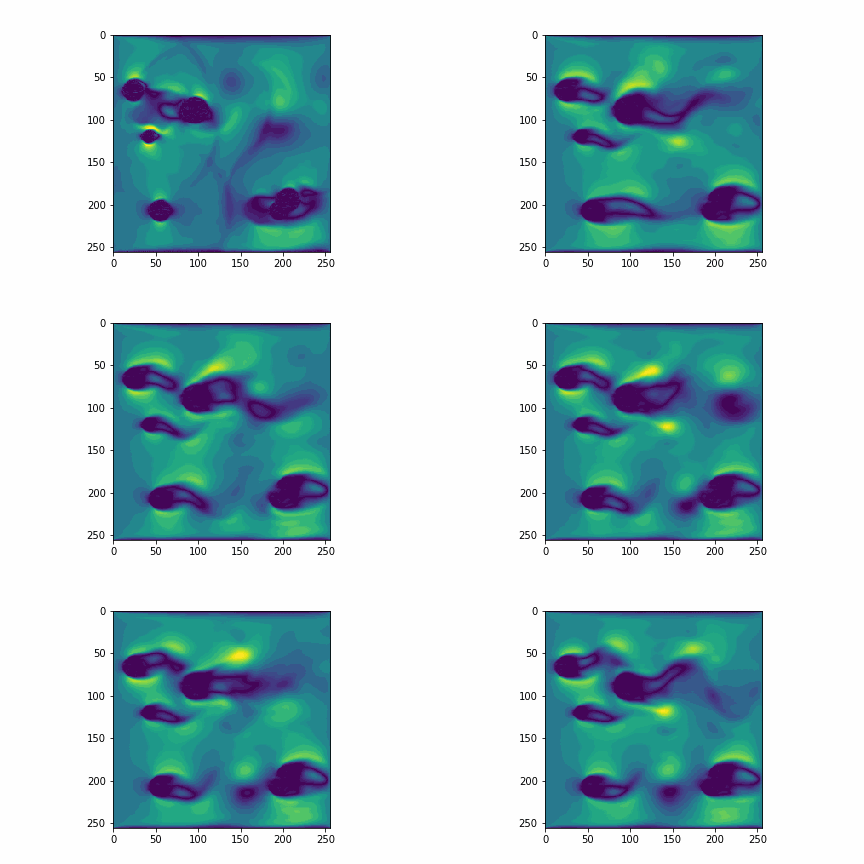
They can be converted to equally scaring functions in code. But they magically create simulations like this:

Despite Machine Learning methods being known for their imprecision, since they try to approximate a function, I decided to try to use them to predict the fluid velocity distribution, because I wanted to learn more about them.

deep learning

The original idea was to use deep learning, given a frame of the simulation, try to predict the next. This simple idea didn't work so well, as it was very computationally expensive to train and also to later use the model on large simulations.

To deal with this, I decided to take a different approach to the problem: instead of using the full frame as input and directly trying to calculate the next frame with them, I decided to split the problem:

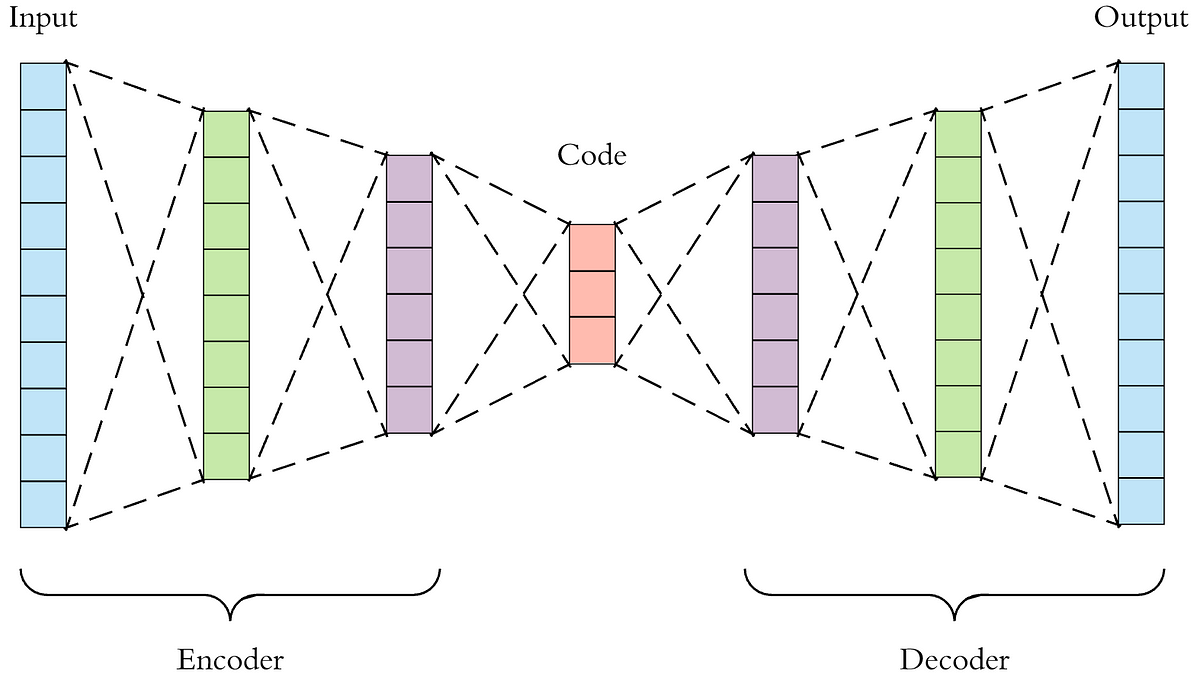
use an encoder to reduce the dimension of the original simulation
use another model responsible only for the physics calculation on this reduced "latent"-space
use a decoder to restore the dimension of this newly generated frame

encoder-decoder neural network architecture — Example of encoder-decoder architecture.

This way, the step number 2 was able to run much faster, given the reduced dimension of the encoded simulation.

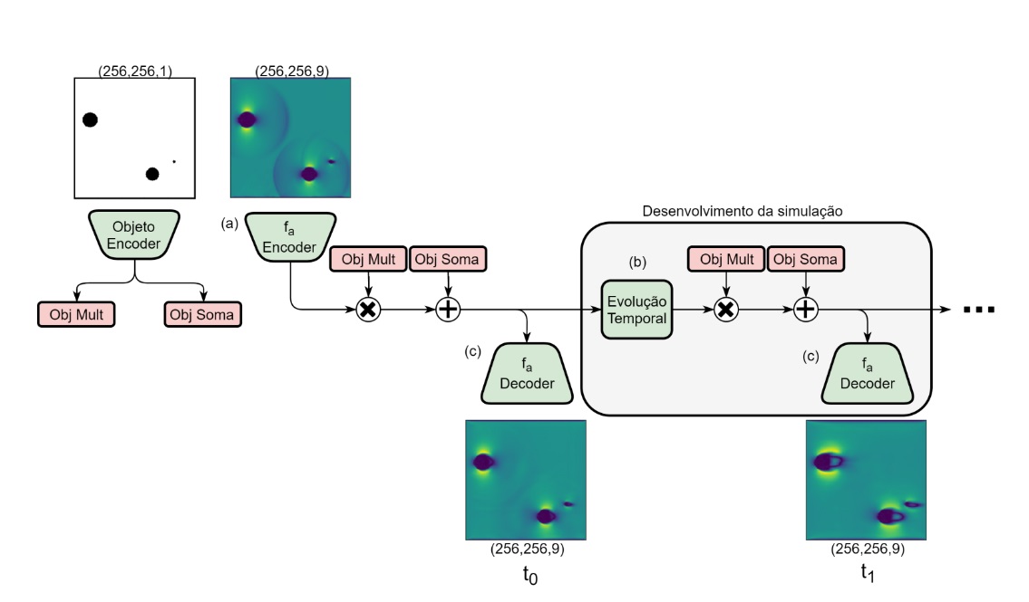
Besides this problem, there was also the case where the obstacles present in the simulations were being corrupted over time, and not correctly persisting in time as they should.

To correct for this, another modification was made, where the objects were also being encoded in two formats: one to multiply the encoded frame, and one to add to the encoded frame. Resulting in the following architecture:

deep learning for fluid dynamics final architecture — Final architecture.

The final result produced nearly visually identical simulations. Due to the challenge that is measuring differences between the simulations, and also due to my focus on Deep Learning, the results weren't so thoroughly compared numerically.

This was one of the first challenging projects I had to deal with, and getting to a working result involved a lot of trial and error, and trying to decipher papers, books and math equations.

In the end I achieved my goal of learning how to better use Python and Tensorflow, allowing me to use these skills later on other projects such as Harpia.